from torch_scatter import scatter
from functools import partial
from typing import Optional, Dict, List
from torch_geometric.datasets import Planetoid
import torch.nn.functional as F
import matplotlib.pyplot as plt
import seaborn as sns
import time

import datetime
dataset = Planetoid(root="tutorial1", name="Cora")
print(f"Cora Graphs, {len(dataset)}")
print(f"Classes: {dataset.num_classes}")
print(f"Features: {dataset.num_features}")Cora Graphs, 1
Classes: 7
Features: 1433Isomorphism: Topologically Identical
Weisfeiler-Lehman Isomorphism Test:
A test to investigate isomorphism in graphs.
\[c_i^{(k)} = h \big(c_i^{(k-1)}, \{c_j^{(k-1)}:j\in\mathcal{N}(i)\} \big)\]
Note: ### \(h\): injective function An injective function is also called a one-to-one function.
Definition: A function \(f\) is injective if it maps distinct inputs to distinct outputs.
i.e. If \(x \ne y\), then \(f(x) \ne f(y)\)
Graph Isomorphism Network (GIN)
It is an attempt to answer whether we can construct a GNN as powerful as the WL Isomorphism test.
\[h_i^{(k)} = \phi(h_i^{(k-1)}, f({h_j^{(k-1)}: j \in \mathcal{N}(i)}))\tag{i}\]
\(k\): Hop-Counter and represents iterative steps or layer number. What it means intuitively is:
\(k=0\): Input features we start with
\(k=1\): The model looks at immediate neighbours
\(k=2\): The model looks at neighbours of neighbours.
The goal remains to select \(\phi\) and \(f\) for are injective
Zaheer et al., (2017) proved that an injective function on multisets can be decomposed as:
\[g(X) = \phi(\sum_{x \in X} f(x))\tag{ii}\]
using (ii), (i) can be expressed as:
\[g(h, X) = \phi\bigg( (1+\epsilon)\cdot f(h) + \sum_{x \in X} f(x)\bigg)\]
we use \(\text{MLP}\) to represent \(\phi\circ f\):
\[h_i^{(k)} = \text{MLP}^{(k)} \bigg((1+\epsilon^{(k)})\cdot h_i^{(k-1)} + \sum_{j\in \mathcal{N}(i)}h_j{(k-1)}\bigg)\]
The authors prove (in the GIN paper) that because MLPs are Universal Approximators, they can model the composition of functions.
MLP=(Linear + ActivationFunct + Linear)
Cons:
- Highly discontinuous function.
No guarantee to find the right function.
Principal Neighborhood Aggregation (PNA)
Primary Idea:
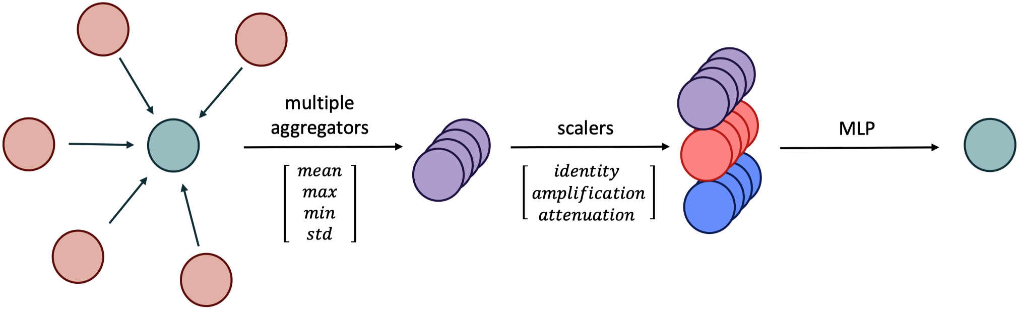
GNNs like Graph Convolution Network (GCN), Graph ATtention GAT, MPNN and GIN use only a single aggregation method with mean, sum and max aggregators being the most used. A limitation of this method is that aggregators fail to discriminate among messages when using a single GNN layer.
To address this, Corso et al. (2020) propose aggregators as continuous functions of multisets. These compute statistics—such as mean, max, or standard deviation—on neighboring nodes. The continuity of input spaces is emphasized: small input changes should yield small output changes for the aggregator.
They used the following aggregators: - Mean Aggregation \(\mu(X^{l})\): The most common message aggregator in the literature, wherein each node computes a weighted average or sum of its incoming messages. This can be calculated as: \[\mu(X^{l}) = \frac{1}{d_i} \sum_{j\in N(i)} X_j^{l}\]
Where $i$: target node, $d_i$: Degree of $i$ node, $j \in N(i)$: all the neighbours of $ i$, $X^{l}$: features vector of a neighbour node $j$ at current layer l.Maximum and Minimum Aggregations: \(\text{max}_i(X^l) = max_{j \in N(i)} X_j^l\), \(\;\;\text{min}_i(X^l) = min_{j \in N(i)} X_j^l\)
Standard Deviation Aggregation: This is calculated as follows:
\[\sigma_i(X^l) = \sqrt{\text{ReLU} \big(\mu_i(X^{l^{2}}) - \mu_i(X^{l}) \big)}\]
Here, mean and standard deviation describe the neighborhood by measuring the average and spread of node features. Higher moments, such as skewness (3rd) and kurtosis (4th), can provide more detail about the neighborhood’s shape. \[\sqrt[n]{\mathbb{E}(X-M)^n}, \;\; n\gt1\]
Degree-based scalers
They also use scalers as functions of the number of messages being aggregated (usually the node degree), which are multiplied by the aggregated value to amplify or attenuate the incoming messages.
\[S = \bigg( \frac{log(d+1)}{\delta} \bigg)^{\alpha}\]
where, \[\delta = \frac{1}{|train|} \sum_{i \in train} log (d_i + 1)\] \(\delta\) is a constant value
\(d\) -> Nodes in the neighbourhood, \(d_i\): Degree of incoming nodes of the neighbours.
\(S_{amp}, \alpha=1\), \(S_{att}, \alpha=-1\), \(S_{identity}\)
Summation aggregation doesn’t generalise well to unseen graphs, as a small change in degree can amplify or attenuate the message and gradients exponentially. In PNA, using a logarithmic amplification \(S \propto log(d+1)\) is proposed to reduce this effect.
\[\bigoplus = \begin{bmatrix} I \\\ S(D, \alpha=1) \\\ S(D, \alpha=-1) \end{bmatrix} \otimes \begin{bmatrix} \mu \\ \sigma \\ \text{max} \\ \text{min} \end{bmatrix}\]
The PNA operator can then be realised in the framework of message passing, which includes edge features also:
\[X_i^{t+1} = U \bigg(X_i^{(t)}, \bigoplus_{(j,i)\in E} (X_i^{(t)}, E_{j \rightarrow i}, X_j^{(t)})\bigg)\]
\(E_{j \rightarrow i}\): is the features of the edge \((j, i)\), \(M\) and \(U\) are neural networks. \(U\): reduces the size of concatenated messages back to \(\mathbb{R}^F\) where \(F\) is the dimension of the hidden features in the network.
import numpy as np
import torch
from torch_geometric.typing import Adj, OptTensor

import torch
from torch import Tensor
from torch.nn import ModuleList, Sequential, Linear, ReLU
from torch_geometric.nn.conv import MessagePassing
from torch_geometric.nn.inits import reset
from torch_geometric.utils import degree, add_self_loops
src_arr = torch.tensor(np.random.randint(0, 100, 10))
indexes = torch.tensor(np.random.randint(0, 3, 10))print('index:', indexes)
print('src arr:', src_arr)index: tensor([1, 0, 0, 1, 2, 0, 0, 0, 1, 1])
src arr: tensor([33, 74, 81, 91, 41, 45, 68, 96, 76, 78])# we use torch_scatter as a mechanism to apply index-wise reduce operation.
reduced_output = scatter(src=src_arr, index=indexes, reduce="sum")
print(reduced_output)tensor([364, 278, 41])Implementation from PNA Repository.
- Aggregators And Scalars using
torch_scatter.scatter
def aggregate_sum(src: Tensor, index: Tensor, dim_size: Optional[int]):
    return scatter(src, index, 0, None, dim_size, reduce='sum')


def aggregate_mean(src: Tensor, index: Tensor, dim_size: Optional[int]):
    return scatter(src, index, 0, None, dim_size, reduce='mean')


def aggregate_min(src: Tensor, index: Tensor, dim_size: Optional[int]):
    return scatter(src, index, 0, None, dim_size, reduce='min')


def aggregate_max(src: Tensor, index: Tensor, dim_size: Optional[int]):
    return scatter(src, index, 0, None, dim_size, reduce='max')


def aggregate_var(src, index, dim_size):
    mean = aggregate_mean(src, index, dim_size)
    mean_squares = aggregate_mean(src * src, index, dim_size)
    return mean_squares - mean * mean


def aggregate_std(src, index, dim_size):
    return torch.sqrt(torch.relu(aggregate_var(src, index, dim_size)) + 1e-5)


AGGREGATORS = {
    'sum': aggregate_sum,
    'mean': aggregate_mean,
    'min': aggregate_min,
    'max': aggregate_max,
    'var': aggregate_var,
    'std': aggregate_std,
}


def scale_identity(src: torch.Tensor, deg: torch.Tensor, avg_deg: Dict[str, float]):
    return src


def scale_amplification(src: torch.Tensor, deg: torch.Tensor, avg_deg: Dict[str, float]):
    return src * (torch.log(deg + 1) / avg_deg['log'])


def scale_attenuation(src: torch.Tensor, deg: torch.Tensor, avg_deg: Dict[str, float]):
    scale = avg_deg['log'] / torch.log(deg + 1)
    scale[deg == 0] = 1
    return src * scale


def scale_linear(src: torch.Tensor, deg: torch.Tensor, avg_deg: Dict[str, float]):
    return src * (deg / avg_deg['lin'])


def scale_inverse_linear(src: torch.Tensor, deg: torch.Tensor, avg_deg: Dict[str, float]):
    scale = avg_deg['lin'] / deg
    scale[deg == 0] = 1
    return src * scale


SCALERS = {
    'identity': scale_identity,
    'amplification': scale_amplification,
    'attenuation': scale_attenuation,
    'linear': scale_linear,
    'inverse_linear': scale_inverse_linear
}- PNAConv Layer Implementation by inheriting
torch_geometric.nn.conv.MessagePassing
class PNAConvSimple(MessagePassing):
    def __init__(self, in_channels: int, out_channels: int,
                 aggregators: List[str], scalers: List[str], deg: Tensor,
                 post_layers: int = 1, **kwargs):
        super(PNAConvSimple, self).__init__(aggr=None, node_dim=0, **kwargs)
        self.in_channels = in_channels #no of input channels
        self.out_channels = out_channels #no
        self.aggregators = [AGGREGATORS[aggr] for aggr in aggregators]
        self.scalars = [SCALERS[scale] for scale in scalers]


        ## see what it does
        self.F_in = in_channels
        self.F_out = out_channels

        deg = deg.to(torch.float)
        total_vertices = deg.sum()
        bin_degrees = torch.arange(len(deg)) # array of size deg
        self.avg_degrees = {
            "lin" : (bin_degrees * deg).sum()/total_vertices,
            "log" : (((bin_degrees +1).log()*deg).sum()/total_vertices).item(), # this is the delta formula in the paper others are generalised versions of it
            "exp" : ((bin_degrees.exp()*deg).sum()/total_vertices).item()
        }
        in_channels = (len(aggregators) * len(scalers)) * self.F_in # 6 * 5 * in_channel

        ## this just stacks MLPs
        modules = [Linear(in_channels, self.F_out)] # just a linear layer
        for _ in range(post_layers-1):
            modules += [ReLU()]
            modules += [Linear(in_channels, self.F_out)]

        self.post_nn = Sequential(*modules)
        self.reset_parameters()

    def reset_parameters(self):
        reset(self.post_nn)

    def forward(self, x: Tensor, edge_index: Adj, edge_attr: OptTensor = None) -> Tensor:

        # propagate_type: (x: Tensor)
        out = self.propagate(edge_index, x=x, size=None)
        return self.post_nn(out)

    def message(self, x_j):
        return x_j

    def aggregate(self, inputs, index, dim_size = None):
        outs = [aggr(inputs, index, dim_size) for aggr in self.aggregators]
        out = torch.cat(outs, dim=-1)
        deg = degree(index, dim_size, dtype=inputs.dtype).view(-1, 1)
        outs = [sclr(out, deg, self.avg_degrees) for sclr in self.scalars]
return torch.cat(outs, dim=-1)- Using
PNAConvSimplein a simple neural network for Node Classification
## Model using GCNN
class PNA_Network(torch.nn.Module):
    def __init__(self, deg_histogram):
        SCALERS = ['identity', 'amplification', 'attenuation', 'linear', 'inverse_linear']
        AGGREGATORS = ['sum', 'mean', 'min', 'max', 'var', 'std']
        super(PNA_Network, self).__init__()
        self.hid = 32
        self.pna_layer = PNAConvSimple(dataset.num_features, dataset.num_classes, AGGREGATORS, SCALERS, deg_histogram)

    def forward(self, data):
        x, edge_index = data.x, data.edge_index
        x = F.dropout(x, p=0.6, training=self.training)
        # print(f"Input shape Conv1: {x.shape}")
        x = self.pna_layer(x, edge_index)

        return F.log_softmax(x, dim=1)
# calculating deg histogram
all_degrees = []
for data in dataset:
all_degrees.append(degree(data.edge_index[0], dtype=torch.long))
all_degrees = torch.cat(all_degrees)
max_degree = all_degrees.max().item()
degree_hist = torch.zeros(max_degree+1, dtype=torch.long)
for deg in all_degrees:
degree_hist[deg] += 1
Degree Histogram
We require degree histogram when using PNA layer for calculating scalars.
sns.set_style('whitegrid')
fig, ax = plt.subplots()
x = np.arange(degree_hist.shape[0])
ax.bar(x, degree_hist)
ax.set_xlabel("Node Degree")
ax.set_ylabel("No. of nodes")
ax.set_title('Degree Histogram')
plt.show()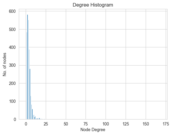
model = PNA_Network(degree_hist)
optimizer = torch.optim.Adam(model.parameters(), lr=0.005, weight_decay=5e-4)
data = dataset[0]
start = time.process_time()
for epoch in range(1000):
model.train()
optimizer.zero_grad()
out = model(data)
loss = F.nll_loss(out[data.train_mask], data.y[data.train_mask])
if epoch%200 == 0:
print(f"Time Elapsed: {time.process_time() - start}, Epoch: {epoch}, loss: {loss.item()}")
loss.backward()
optimizer.step()Time Elapsed: 2.681476000000001, Epoch: 0, loss: 1.9427117109298706
Time Elapsed: 483.15815299999997, Epoch: 200, loss: 0.012473355047404766
Time Elapsed: 965.493997, Epoch: 400, loss: 0.011228213086724281
Time Elapsed: 1449.137884, Epoch: 600, loss: 0.06128396838903427
Time Elapsed: 1929.509851, Epoch: 800, loss: 0.001116628060117364GIN Implementation
If all Aggregators except sum are removed and the central node is added using self loops. The PNA implementation can be reduced to an instance of GIN layer.
class GINConvSimple(MessagePassing):
    def __init__(self, in_channels: int, out_channels: int,
                 post_layers: int = 1, **kwargs):
        super(GINConvSimple, self).__init__(aggr=None, node_dim=0, **kwargs)
        self.in_channels = in_channels #no of input channels
        self.out_channels = out_channels #no

        # reducing aggregators to sum
        self.aggregators = [AGGREGATORS[aggr] for aggr in ['sum']]


        ## see what it does
        self.F_in = in_channels
        self.F_out = out_channels


        in_channels = (1 * 1) * self.F_in # 6 * 5 * in_channel #adjustment based on scalars

        ## this just stacks MLPs
        modules = [Linear(in_channels, self.F_out)] # just a linear layer
        for _ in range(post_layers-1):
            modules += [ReLU()]
            modules += [Linear(in_channels, self.F_out)]

        self.post_nn = Sequential(*modules)
        self.reset_parameters()

    def reset_parameters(self):
        reset(self.post_nn)

    def forward(self, x: Tensor, edge_index: Adj, edge_attr: OptTensor = None) -> Tensor:

        # propagate_type: (x: Tensor)
        edge_index, _ = add_self_loops(edge_index)
        out = self.propagate(edge_index, x=x, size=None)
        return self.post_nn(out)

    def message(self, x_j):
        return x_j

    def aggregate(self, inputs, index, dim_size = None):
        outs = [aggr(inputs, index, dim_size) for aggr in self.aggregators]

        out = torch.cat(outs, dim=-1)

        # deg = degree(index, dim_size, dtype=inputs.dtype).view(-1, 1)
        # outs = [sclr(out, deg, self.avg_degrees) for sclr in self.scalars]
        return out


class GIN_Network(torch.nn.Module):
    def __init__(self):

        super(GIN_Network, self).__init__()
        self.hid = 32
        self.pna_layer = GINConvSimple(dataset.num_features, dataset.num_classes)

    def forward(self, data):
        x, edge_index = data.x, data.edge_index
        x = F.dropout(x, p=0.6, training=self.training)
        # print(f"Input shape Conv1: {x.shape}")
        x = self.pna_layer(x, edge_index)

        return F.log_softmax(x, dim=1)
model = GIN_Network()
optimizer = torch.optim.Adam(model.parameters(), lr=0.005, weight_decay=5e-4)
data = dataset[0]start = time.process_time()
for epoch in range(1000):
model.train()
optimizer.zero_grad()
out = model(data)
loss = F.nll_loss(out[data.train_mask], data.y[data.train_mask])
if epoch%200 == 0:
print(f"Time Elapsed: {time.process_time() - start}, Epoch: {epoch}, loss: {loss.item()}")
loss.backward()
optimizer.step()Time Elapsed: 0.2294729999998708, Epoch: 0, loss: 1.9651533365249634
Time Elapsed: 62.08905800000002, Epoch: 200, loss: 0.02035176381468773
Time Elapsed: 124.28675900000007, Epoch: 400, loss: 0.012289958074688911
Time Elapsed: 186.90790199999992, Epoch: 600, loss: 0.011557257734239101
Time Elapsed: 248.96050700000023, Epoch: 800, loss: 0.01037731021642685NOTE
The layers discussed are simplistic implementations for ease of understanding. In real-world scenarios, the use of PyTorch geometric implementation is recommended.
Pytorch Geometric Implementations - LINK